Introduction
Class midpoints serve as the heart of statistical analysis. They represent the central value of a class interval in a frequency distribution, making them essential for summarizing data. Think of them as the friendly neighborhood guide that helps us navigate through groups of data points.
Understanding class midpoints is crucial. They provide insight into frequency distributions, allowing for better data visualization and analysis. Whether you’re crafting histograms or calculating averages, these midpoints simplify the process and enhance accuracy.
This article aims to be your go-to resource on finding class midpoints. We’ll walk you through a step-by-step guide, complete with examples and applications. Plus, we’ve included additional resources to deepen your understanding. Ready to become a class midpoint pro? Let’s get started!

Understanding Class Midpoints
What is a Class Midpoint?
A class midpoint, also known as a class mark, is the average of the upper and lower limits of a class interval. Picture this: if you have a class interval of 10-20, the midpoint is simply (10 + 20) / 2, which equals 15. Easy, right?
Class midpoints play a vital role in statistics, especially in frequency distributions. They provide a single representative value for all data points within a class, making it easier to analyze and interpret data. When we plot a histogram, each bar is centered at its respective class midpoint, allowing for a clearer visual representation of the data.
Why are Class Midpoints Important?
Class midpoints are not just numbers; they’re valuable tools in statistical analyses. They help in calculating measures of central tendency, such as the mean. For instance, when calculating the mean of a dataset represented by a frequency distribution, midpoints streamline the process.
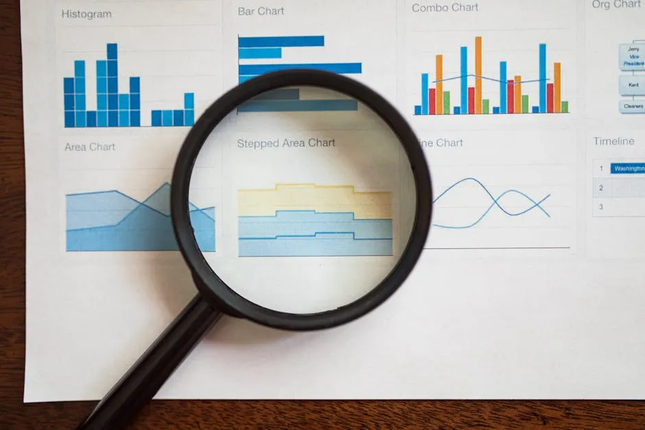
Consider a histogram. The x-axis represents the class intervals, while the y-axis shows the frequency of each class. Each bar sits pretty at its class midpoint, offering a snapshot of the data distribution. This visualization aids in spotting trends and patterns at a glance.
Applications extend beyond histograms. Midpoints assist in calculating weighted means, where each midpoint is multiplied by its corresponding frequency. This calculation is essential when working with grouped data, ensuring accuracy and efficiency.
In summary, class midpoints are instrumental in statistics. They simplify data analysis, enhance the clarity of visual representations, and facilitate calculations. Understanding their significance is key to mastering statistical concepts and effectively communicating data insights.

Step-by-Step Guide to Finding Class Midpoints
Finding class midpoints is essential in statistics, especially when analyzing frequency distributions. This guide will walk you through two crucial steps: identifying class intervals and calculating midpoints. So grab a cup of coffee, and let’s get to it!
If you’re gearing up for this journey into the world of statistics, you might want to equip yourself with some handy tools! A Graphing Calculator can make calculations a breeze, allowing you to focus on understanding the concepts rather than getting bogged down with arithmetic.

Step 1: Identify Class Intervals
First things first, what are class intervals? They are simply ranges of values grouped together in a frequency distribution table. Think of them as the cozy homes where data points like to hang out.
To identify class intervals from a frequency distribution table, look for the lower and upper limits of each class. Here’s a sample frequency distribution table for reference:
| Class | Frequency |
|---|---|
| 1 – 10 | 20 |
| 11 – 20 | 21 |
| 21 – 30 | 16 |
| 31 – 40 | 5 |
| 41 – 50 | 4 |
From this table, we can see five distinct class intervals: 1-10, 11-20, 21-30, 31-40, and 41-50. Each interval represents a range of values, with the first number being the lower limit and the second the upper limit. If you’re wondering why this matters, it’s because knowing these intervals sets the stage for calculating midpoints!

Step 2: Calculate the Midpoint for Each Class Interval
Now that we have our intervals, it’s time to calculate the midpoints. The formula is simple:
Midpoint = (Lower Class Limit + Upper Class Limit) / 2
Let’s break down the calculation process with some examples.

Example 1: Class Interval 1-10
– Lower Class Limit: 1
– Upper Class Limit: 10
Applying the formula:
Midpoint = (1 + 10) / 2 = 11 / 2 = 5.5
Example 2: Class Interval 21-30
– Lower Class Limit: 21
– Upper Class Limit: 30
Using the same formula:
Midpoint = (21 + 30) / 2 = 51 / 2 = 25.5
Now, let’s summarize the midpoints for all class intervals in our example frequency distribution table:
| Class | Frequency | Midpoint |
|---|---|---|
| 1 – 10 | 20 | 5.5 |
| 11 – 20 | 21 | 15.5 |
| 21 – 30 | 16 | 25.5 |
| 31 – 40 | 5 | 35.5 |
| 41 – 50 | 4 | 45.5 |
And just like that, we have a complete table with midpoints calculated for each class interval!

Example Problem
Let’s put our newfound knowledge into practice with a complete example problem. Here’s the frequency distribution table again for clarity:
| Class | Frequency |
|---|---|
| 1 – 10 | 20 |
| 11 – 20 | 21 |
| 21 – 30 | 16 |
| 31 – 40 | 5 |
| 41 – 50 | 4 |
1. Identify the class intervals: We already have them listed above.
2. Calculate the midpoints:
– For 1-10: (1 + 10) / 2 = 5.5
– For 11-20: (11 + 20) / 2 = 15.5
– For 21-30: (21 + 30) / 2 = 25.5
– For 31-40: (31 + 40) / 2 = 35.5
– For 41-50: (41 + 50) / 2 = 45.5
Now, we compile everything into a summary table:
| Class | Frequency | Midpoint |
|---|---|---|
| 1 – 10 | 20 | 5.5 |
| 11 – 20 | 21 | 15.5 |
| 21 – 30 | 16 | 25.5 |
| 31 – 40 | 5 | 35.5 |
| 41 – 50 | 4 | 45.5 |
And there you have it! You’ve successfully calculated the midpoints for each class interval. These midpoints will be invaluable for further statistical analysis, from constructing histograms to calculating means.
Now that you’ve mastered these steps, you’re one step closer to becoming a statistics whiz! Stay tuned for the next part of our guide, where we’ll show you how to compile these midpoints into a summary table for even better data visualization. Happy calculating!

Step 3: Compile Midpoints into a Summary Table
Now that you’ve calculated the midpoints for each class interval, it’s time to compile them into a summarized table. This table will not only include the midpoints but also the corresponding class intervals and frequencies. A well-organized summary table is your best friend in statistical analysis. It allows you to see your data at a glance, making it easier to draw insights and conclusions.
Here’s how to create your summary table:
- List the Class Intervals: Start by writing down all the class intervals you’ve identified. Each interval should be clearly defined, such as “1-10” or “21-30.”
- Include Frequencies: Next to each class interval, write down its corresponding frequency. This number indicates how many data points fall within that interval.
- Add Midpoints: Finally, include the midpoints you’ve calculated for each class interval. This will help visualize the central tendency of each class.
Let’s take a look at a visual representation:
| Class | Frequency | Midpoint |
|---|---|---|
| 1 – 10 | 20 | 5.5 |
| 11 – 20 | 21 | 15.5 |
| 21 – 30 | 16 | 25.5 |
| 31 – 40 | 5 | 35.5 |
| 41 – 50 | 4 | 45.5 |
This summary table provides a clear overview of the data. It highlights how many observations are in each interval and where the midpoint lies, making it an essential tool for any further statistical analysis.

Applications of Class Midpoints
Using Class Midpoints in Histograms
Class midpoints are crucial when constructing histograms. Imagine trying to create a visual representation of your data without knowing where to place the bars! Midpoints act as the anchor points for these bars. Each bar in a histogram represents a class interval, with its height corresponding to the frequency of that interval.
When plotting, ensure that each bar is centered at its respective midpoint. This accurate placement is vital for an effective histogram. If bars are misplaced, the visual representation can be misleading, leading to incorrect interpretations.
For example, if you have a class interval of 11-20, the midpoint is 15.5. The bar for this interval should be centered around this value on the x-axis. Doing so allows viewers to quickly grasp the distribution of data across intervals, making trends and patterns easier to identify at a glance.

Importance in Further Statistical Analysis
Class midpoints are not just pretty faces on a histogram; they also play a significant role in calculating measures of central tendency, such as the weighted mean. The weighted mean gives greater importance to certain values based on their frequency, making it a more accurate representation of the dataset.
Here’s a quick example of calculating a weighted mean using midpoints:
Suppose you have the following data:
| Class | Frequency | Midpoint |
|---|---|---|
| 1 – 10 | 20 | 5.5 |
| 11 – 20 | 21 | 15.5 |
| 21 – 30 | 16 | 25.5 |
To compute the weighted mean, follow these steps:
- Multiply each midpoint by its corresponding frequency:
– 5.5 x 20 = 110
– 15.5 x 21 = 325.5
– 25.5 x 16 = 408 - Add these products together:
– Total = 110 + 325.5 + 408 = 843.5 - Sum the frequencies:
– Total Frequency = 20 + 21 + 16 = 57 - Finally, divide the total of the products by the total frequency:
– Weighted Mean = 843.5 / 57 ≈ 14.81
This weighted mean provides a more accurate representation of your data’s central tendency, showcasing how midpoints can be instrumental in further statistical analysis. By understanding the applications of class midpoints, you’re not just crunching numbers; you’re optimizing your data analysis skills!

Common Mistakes and Misunderstandings
Misinterpretation of Class Boundaries
When working with class midpoints, confusion often arises around class boundaries. Many might assume that class intervals, like 10-20, encompass values strictly between 10 and 20. In reality, these intervals include the lower limit but exclude the upper limit, effectively representing the range from 10 to just below 20. This misunderstanding can lead to incorrect midpoint calculations.
For instance, the class interval 10-20 should have a midpoint calculated as follows:
Incorrect Calculation:
– Midpoint = (10 + 20) / 2 = 15
This calculation seems logical, but it misrepresents the class. Instead, it would be more accurate to evaluate the midpoint like this:
Correct Calculation:
– Midpoint = (10 + 19.999…) / 2 = 14.999…
This minor adjustment highlights the importance of understanding class boundaries. Always remember that precise calculations hinge on the correct interpretation of these limits.

Overlooking Open-ended Classes
Open-ended classes, such as 50 and above, present unique challenges. With no definitive upper limit, calculating midpoints can feel like trying to hit a moving target. The key is to apply reasonable assumptions.
One common approach is to take the width of the adjacent classes into account. For example, if the previous class interval is 40-50, you can assume that your open-ended class maintains the same width. If the last class is 40-50, you can calculate the midpoint for 50 and above using this width as a guide.
For instance:
– Assume the width of the class is 10 (from 40-50).
– You can define the open-ended class as 50-60 for calculations.
– Thus, the midpoint would be (50 + 60) / 2 = 55.
This methodology allows for a more structured approach to open-ended classes, ensuring your midpoint calculations remain as accurate as possible.
Additional Resources
To enhance your understanding of class midpoints and statistics in general, consider these resources:
- Books on Statistics: Look for titles like “Statistics for Dummies” or “The Art of Statistics” for foundational insights and practical applications.
- Online Courses: Platforms like Coursera and edX offer courses on statistics that cover concepts from basic to advanced levels, including class midpoints and frequency distributions.
- Interactive Websites: Websites such as Statology and Mathway provide calculators for finding midpoints and visual aids for understanding frequency distributions. These tools simplify learning by allowing you to input data and see results instantly.
By leveraging these resources, you can deepen your comprehension of statistical concepts and improve your practical skills in calculating class midpoints.
If you’re serious about diving deeper into data analysis, consider grabbing a copy of the Statistical Analysis System (SAS) Essentials Book. It’s a must-read for anyone looking to master statistical software!

Conclusion
In this guide, we’ve journeyed through the world of class midpoints in statistics. These midpoints are more than just numbers; they serve as critical tools for understanding data distributions. We kicked off by defining class midpoints and their importance in frequency distributions. We highlighted how they simplify data analysis and aid in calculating key statistical measures, such as the mean.
We also detailed a step-by-step process for finding class midpoints, from identifying class intervals to calculating and compiling them into a summary table. This structured approach ensures that no data point goes unnoticed, making your statistical analysis robust and reliable.
Understanding and accurately calculating class midpoints is vital for anyone diving into statistics, whether for academic purposes or data analysis in the workplace. It enhances your ability to visualize data effectively, paving the way for informed decision-making.
Now, don’t just take our word for it! Practice makes perfect. We encourage you to tackle additional examples and reinforce your newfound skills. The more you practice, the more proficient you’ll become in using class midpoints to turn raw data into meaningful insights.

FAQs
What is the formula for calculating class midpoints?
Calculating class midpoints is straightforward! The formula is: \[ \text{Midpoint} = \frac{\text{Lower Class Limit} + \text{Upper Class Limit}}{2} \] Let’s take a look at an example. If you have a class interval of 10-20, the calculation would be: \[ \text{Midpoint} = \frac{10 + 20}{2} = 15 \] So, for the class interval of 10-20, the midpoint is 15.
How do you find midpoints for open-ended classes?
Open-ended classes can be tricky because they lack a defined upper or lower limit. For example, consider a class like “50 and above.” In such cases, you can estimate the midpoint by assuming the class has the same width as adjacent classes. For instance, if the previous class is “40-50,” you could consider the open-ended class as “50-60” for calculation purposes. Then, the midpoint would be: \[ \text{Midpoint} = \frac{50 + 60}{2} = 55 \] This method helps provide a reasonable estimate for the midpoint in open-ended situations.
Can class midpoints be used for non-numeric data?
Class midpoints are primarily designed for numeric data, where they represent central values within defined ranges. However, in categorical datasets, midpoints can offer insights if numerical values are assigned to categories. For example, if you categorize responses into “Low,” “Medium,” and “High,” you might assign values like 1, 2, and 3, respectively. While it’s not a perfect fit, you can use these values to calculate a sort of midpoint for analysis. Just remember, this approach should be used cautiously, as it may not perfectly represent the data’s nature.
What are class boundaries, and how do they relate to midpoints?
Class boundaries define the limits between different classes in a frequency distribution. They help ensure that classes do not overlap and assist in accurate calculations. The lower class boundary is the average of the upper limit of the previous class and the lower limit of the current class. The upper class boundary is calculated similarly. For example, in the class interval “10-20”: The lower boundary is 9.5 (average of 10 and 9). The upper boundary is 20.5 (average of 20 and 21). Understanding class boundaries is essential for calculating accurate midpoints, ensuring that your data interpretation is spot-on.
How are midpoints useful in calculating the mean?
Midpoints simplify the process of finding the mean in grouped data. Instead of using every individual data point, you can use the midpoints of each class multiplied by their respective frequencies. Here’s how it works: 1. Multiply each midpoint by the class frequency. 2. Sum these products. 3. Divide by the total frequency to obtain the mean. For example, if you have midpoints of 5.5, 15.5, and 25.5 with frequencies of 20, 21, and 16, respectively: Calculate the products: \(5.5 \times 20 = 110\), \(15.5 \times 21 = 325.5\), \(25.5 \times 16 = 408\). Add them: Total = \(110 + 325.5 + 408 = 843.5\). Total frequency = \(20 + 21 + 16 = 57\). Finally, divide: \( \frac{843.5}{57} \approx 14.81\). And just like that, midpoints make finding the mean less of a headache!
Please let us know what you think about our content by leaving a comment down below!
Thank you for reading till here 🙂
For a deeper understanding of how to effectively summarize data, consider checking out this statistical summary table.
All images from Pexels


